Wavelet Frequency Spacing
Frequently, using a fixed ratio for scaling the wavelets results in too many large scale wavelets. There are several ways of dealing with this; in this package, the scaling factors have the form $2^{x_0 +mx^{^1/_\beta}}$, for suitable choice of $a$,$m$, $x_0$, and $\beta$. The user chooses $\beta$ and $Q$, and the rest are chosen to match the derivative at the last frequency to be $^{1}/_{Q}$, as in the figure.

If $\beta$ is 1, then we have a linear relation between the index and the log-frequency, and $Q$ gives exactly the number of wavelets per octave throughout. As $\beta$ increases, the wavelets skew more and more heavily to high frequencies. The default value is 4.
The user chooses β (the frequency decay), Q (the number of wavelets per octave at the last point), and aveLen (the number of octaves covered by the averaging function, here $x_0$), and then $m$, the number of wavelets $N_w$, and the spacing of $x$ are chosen so that:
- The derivative $\frac{\mathrm{d}y}{\mathrm{d}x}$ at the last point is $^{1}/_{Q}$, so the "instantaneous" number of wavelets $x$ per octave $y$ is $Q$. Each type of wavelet has a maximum scaling $2^{N_{Octaves}}$ returned by
getNOctaves(generally half the signal length), so the final point $N_w$ satisfies both $y(N_w) = N_{Octaves}$ and $y'(N_w)=^1/_Q$. - The spacing is chosen so that there are exactly $Q$ wavelets in the last octave.
If you are interested in the exact computation, see the function polySpacing. As some examples of how the wavelet bank changes as we change $\beta$:
n=2047
Ψ1 = wavelet(morl, s=8, β=1)
d1, ξ = computeWavelets(n,Ψ1)
Ψ2 = wavelet(morl, s=8, β =2)
d2, ξ = computeWavelets(n,Ψ2)
Ψ4 = wavelet(morl, s=8, β =4)
d4, ξ = computeWavelets(n,Ψ4)
plot(heatmap(1:size(d1,2), ξ, d1, color=:Greys, yaxis = (L"\omega", ), xaxis = ("wavelet index", ), title=L"\beta=1"*" ("*L"\Psi1"*")", colorbar=false, clims=matchingLimits),  heatmap(1:size(d2,2), ξ, d2, color=:Greys, yticks=[], xaxis = ("wavelet index", ), title=L"\beta=2"*" ("*L"\Psi2"*")", colorbar=false, clims=matchingLimits),  heatmap(1:size(d4,2), ξ, d4,color=:Greys, yticks=[], xticks=[1, 5, 10, 14, 18], xaxis = ("wavelet index", ), title=L"\beta=4"*" ("*L"\Psi4"*")"), layout=(1,3), clims=matchingLimits, colorbar_title=L"\widehat{\psi_i}")
"/home/runner/work/ContinuousWavelets.jl/ContinuousWavelets.jl/docs/build/changeBeta.png"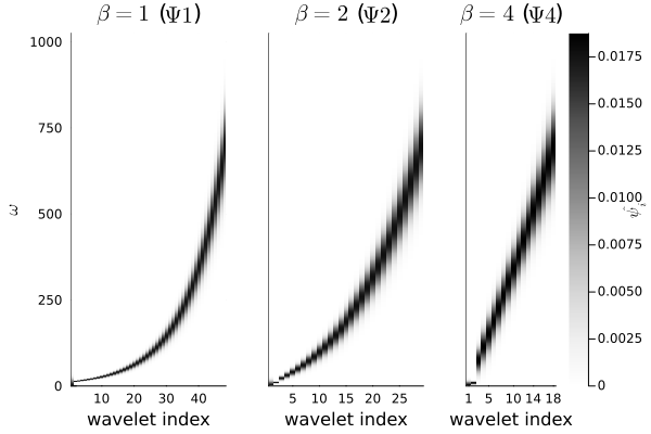
note that the low-frequency coverage increases drastically as we decrease $\beta$.